
Topology optimisation of fluids in Stokes flow
Section author: Patrick E. Farrell <patrick.farrell@maths.ox.ac.uk>
This demo solves example 4 of [4E-BP03].
Problem definition
This problem is to minimise the dissipated power in the fluid
subject to the Stokes equations with velocity Dirichlet conditions
and to the control constraints on available fluid volume
where \(u\) is the velocity, \(p\) is the pressure, \(\rho\) is the control (\(\rho(x) = 1\) means fluid present, \(\rho(x) = 0\) means no fluid present), \(f\) is a prescribed source term (here 0), \(V\) is the volume bound on the control, \(\alpha(\rho)\) models the inverse permeability as a function of the control
with \(\bar{\alpha}\), \(\underline{\alpha}\) and \(q\) prescribed constants. The parameter \(q\) penalises deviations from the values 0 or 1; the higher q, the closer the solution will be to having the two discrete values 0 or 1.
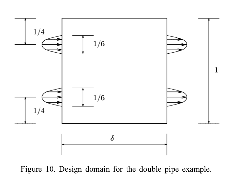
The problem domain \(\Omega\) is parameterised by the aspect ratio \(\delta\) (the domain is 1 unit high and \(\delta\) units wide); in this example, we will solve the harder problem of \(\delta = 1.5\). The boundary conditions are specified in figure 10 of Borrvall and Petersson, reproduced here.
Physically, this problem corresponds to finding the fluid-solid distribution \(\rho(x)\) that minimises the dissipated power in the fluid.
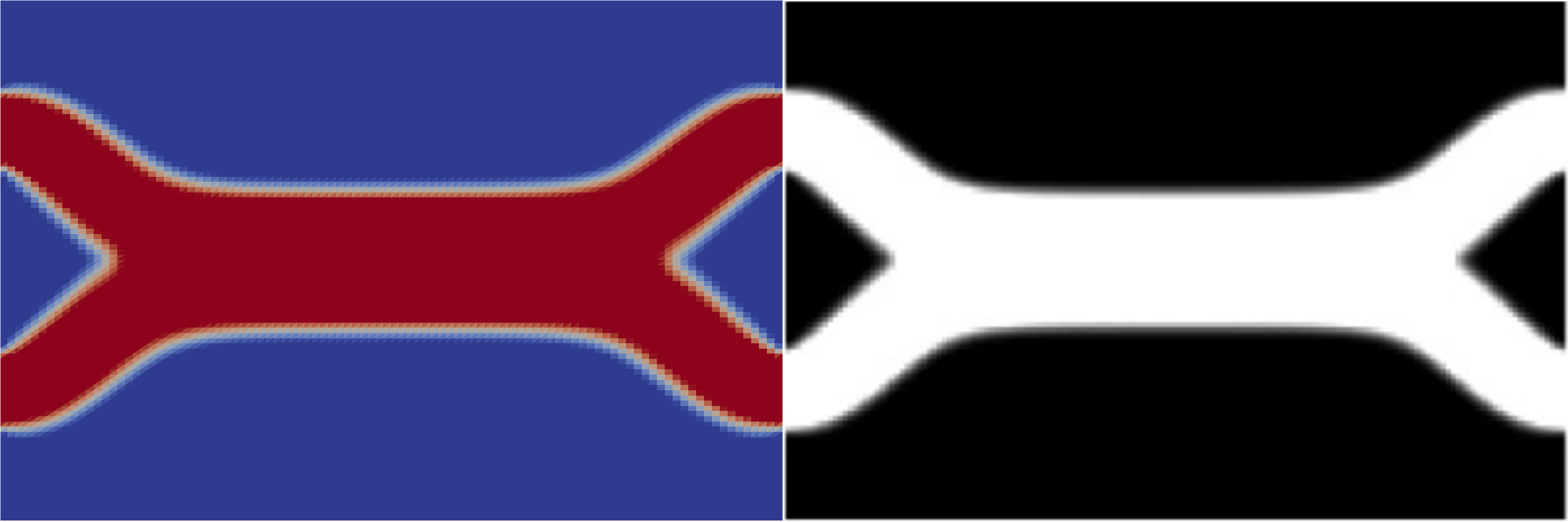
As Borrvall and Petersson comment, it is necessary to solve this problem with \(q=0.1\) to ensure that the result approaches a discrete-valued solution, but solving this problem directly with this value of \(q\) leads to a local minimum configuration of two straight pipes across the domain (like the top half of figure 11). Therefore, we follow their suggestion to first solve the optimisation problem with a smaller penalty parameter of \(q=0.01\); this optimisation problem does not yield bang-bang solutions but is easier to solve, and gives an initial guess from which the \(q=0.1\) case converges to the better minimum.
Implementation
First, the dolfin and dolfin_adjoint modules are
imported:
from __future__ import print_function
from dolfin import *
from dolfin_adjoint import *
Next we import the Python interface to IPOPT. If IPOPT is unavailable on your system, we strongly suggest you install it; IPOPT is a well-established open-source optimisation algorithm.
try:
    import pyipopt
except ImportError:
    info_red("""This example depends on IPOPT and pyipopt. \
  When compiling IPOPT, make sure to link against HSL, as it \
  is a necessity for practical problems.""")
    raise

# turn off redundant output in parallel
parameters["std_out_all_processes"] = False
Next we define some constants, and define the inverse permeability as a function of \(\rho\).
mu = Constant(1.0)                   # viscosity
alphaunderbar = 2.5 * mu / (100**2)  # parameter for \alpha
alphabar = 2.5 * mu / (0.01**2)      # parameter for \alpha
q = Constant(0.01) # q value that controls difficulty/discrete-valuedness of solution

def alpha(rho):
    """Inverse permeability as a function of rho, equation (40)"""
    return alphabar + (alphaunderbar - alphabar) * rho * (1 + q) / (rho + q)
Next we define the mesh (a rectangle 1 high and \(\delta\) wide) and the function spaces to be used for the control \(\rho\), the velocity \(u\) and the pressure \(p\). Here we will use the Taylor-Hood finite element to discretise the Stokes equations [4E-TH73].
N = 200
delta = 1.5  # The aspect ratio of the domain, 1 high and \delta wide
V = Constant(1.0/3) * delta  # want the fluid to occupy 1/3 of the domain

mesh = RectangleMesh(mpi_comm_world(), Point(0.0, 0.0), Point(delta, 1.0), N, N)
A = FunctionSpace(mesh, "CG", 1)        # control function space

U_h = VectorElement("CG", mesh.ufl_cell(), 2)
P_h = FiniteElement("CG", mesh.ufl_cell(), 1)
W = FunctionSpace(mesh, U_h*P_h)          # mixed Taylor-Hood function space
Define the boundary condition on velocity
class InflowOutflow(Expression):
    def eval(self, values, x):
        values[1] = 0.0
        values[0] = 0.0
        l = 1.0/6.0
        gbar = 1.0

        if x[0] == 0.0 or x[0] == delta:
            if (1.0/4 - l/2) < x[1] < (1.0/4 + l/2):
                t = x[1] - 1.0/4
                values[0] = gbar*(1 - (2*t/l)**2)
            if (3.0/4 - l/2) < x[1] < (3.0/4 + l/2):
                t = x[1] - 3.0/4
                values[0] = gbar*(1 - (2*t/l)**2)

    def value_shape(self):
        return (2,)
Next we define a function that given a control \(\rho\) solves the forward PDE for velocity and pressure \((u, p)\). (The advantage of formulating it in this manner is that it makes it easy to conduct Taylor remainder convergence tests.)
def forward(rho):
    """Solve the forward problem for a given fluid distribution rho(x)."""
    w = Function(W)
    (u, p) = split(w)
    (v, q) = TestFunctions(W)

    F = (alpha(rho) * inner(u, v) * dx + inner(grad(u), grad(v)) * dx +
         inner(grad(p), v) * dx  + inner(div(u), q) * dx)
    bc = DirichletBC(W.sub(0), InflowOutflow(), "on_boundary")
    solve(F == 0, w, bcs=bc)

    return w
Now we define the __main__ section. We define the initial guess
for the control and use it to solve the forward PDE. In order to
ensure feasibility of the initial control guess, we interpolate the
volume bound; this ensures that the integral constraint and the bound
constraint are satisfied.
if __name__ == "__main__":
    rho = interpolate(Constant(float(V)/delta), A, name="Control")
    w   = forward(rho)
    (u, p) = split(w)
With the forward problem solved once, dolfin_adjoint has
built a tape of the forward model; it will use this tape to drive
the optimisation, by repeatedly solving the forward model and the
adjoint model for varying control inputs.
As in the Poisson topology example, we will use an evaluation
callback to dump the control iterates to disk for visualisation. As
this optimisation problem (\(q=0.01\)) is solved only to generate
an initial guess for the main task (\(q=0.1\)), we shall save
these iterates in output/control_iterations_guess.pvd.
controls = File("output/control_iterations_guess.pvd")
allctrls = File("output/allcontrols.pvd")
rho_viz = Function(A, name="ControlVisualisation")
def eval_cb(j, rho):
    rho_viz.assign(rho)
    controls << rho_viz
    allctrls << rho_viz
Now we define the functional and reduced functional:
J = Functional(0.5 * inner(alpha(rho) * u, u) * dx + mu * inner(grad(u), grad(u)) * dx)
m = Control(rho)
Jhat = ReducedFunctional(J, m, eval_cb_post=eval_cb)
The control constraints are the same as the Poisson topology example, and so won’t be discussed again here.
# Bound constraints
lb = 0.0
ub = 1.0

# Volume constraints
class VolumeConstraint(InequalityConstraint):
    """A class that enforces the volume constraint g(a) = V - a*dx >= 0."""
    def __init__(self, V):
        self.V = float(V)
The derivative of the constraint g(x) is constant (it is the negative of the diagonal of the lumped mass matrix for the control function space), so let’s assemble it here once. This is also useful in rapidly calculating the integral each time without re-assembling.
    self.smass = assemble(TestFunction(A) * Constant(1) * dx)
    self.tmpvec = Function(A)

def function(self, m):
    print("Evaluting constraint residual")
    self.tmpvec.vector()[:] = m

    # Compute the integral of the control over the domain
    integral = self.smass.inner(self.tmpvec.vector())
    print("Current control integral: ", integral)
    return [self.V - integral]

def jacobian(self, m):
    print("Computing constraint Jacobian")
    return [-self.smass]

def output_workspace(self):
    return [0.0]
Now that all the ingredients are in place, we can perform the initial optimisation. We set the maximum number of iterations for this initial optimisation problem to 30; there’s no need to solve this to completion, as its only purpose is to generate an initial guess.
# Solve the optimisation problem with q = 0.01
problem = MinimizationProblem(Jhat, bounds=(lb, ub), constraints=VolumeConstraint(V))
parameters = {'maximum_iterations': 20}

solver = IPOPTSolver(problem, parameters=parameters)
rho_opt = solver.solve()

rho_opt_xdmf = XDMFFile(mpi_comm_world(), "output/control_solution_guess.xdmf")
rho_opt_xdmf.write(rho_opt)
With the optimised value for \(q=0.01\) in hand, we reset the dolfin-adjoint state, clearing its tape, and configure the new problem we want to solve. We need to update the values of \(q\) and \(\rho\):
q.assign(0.1)
rho.assign(rho_opt)
adj_reset()
Since we have cleared the tape, we need to execute the forward model
once again to redefine the problem. (It is also possible to modify the
tape, but this way is easier to understand.) We will also redefine the
functionals and parameters; this time, the evaluation callback will
save the optimisation iterations to
output/control_iterations_final.pvd.
rho_intrm = XDMFFile(mpi_comm_world(), "intermediate-guess-%s.xdmf" % N)
rho_intrm.write(rho)

w = forward(rho)
(u, p) = split(w)

# Define the reduced functionals
controls = File("output/control_iterations_final.pvd")
rho_viz = Function(A, name="ControlVisualisation")
def eval_cb(j, rho):
    rho_viz.assign(rho)
    controls << rho_viz
    allctrls << rho_viz

J = Functional(0.5 * inner(alpha(rho) * u, u) * dx + mu * inner(grad(u), grad(u)) * dx)
m = Control(rho)
Jhat = ReducedFunctional(J, m, eval_cb_post=eval_cb)
We can now solve the optimisation problem with \(q=0.1\), starting from the solution of \(q=0.01\):
problem = MinimizationProblem(Jhat, bounds=(lb, ub), constraints=VolumeConstraint(V))
parameters = {'maximum_iterations': 100}

solver = IPOPTSolver(problem, parameters=parameters)
rho_opt = solver.solve()

rho_opt_final = XDMFFile(mpi_comm_world(), "output/control_solution_final.xdmf")
rho_opt_final.write(rho_opt)
The example code can be found in examples/stokes-topology/ in the
dolfin-adjoint source tree, and executed as follows:
$ mpiexec -n 4 python stokes-topology.py
...
Number of Iterations....: 100

                                   (scaled)                 (unscaled)
Objective...............:   4.5944633030224409e+01    4.5944633030224409e+01
Dual infeasibility......:   1.8048641504211900e-03    1.8048641504211900e-03
Constraint violation....:   0.0000000000000000e+00    0.0000000000000000e+00
Complementarity.........:   9.6698653740681504e-05    9.6698653740681504e-05
Overall NLP error.......:   1.8048641504211900e-03    1.8048641504211900e-03


Number of objective function evaluations             = 105
Number of objective gradient evaluations             = 101
Number of equality constraint evaluations            = 0
Number of inequality constraint evaluations          = 105
Number of equality constraint Jacobian evaluations   = 0
Number of inequality constraint Jacobian evaluations = 101
Number of Lagrangian Hessian evaluations             = 0
Total CPU secs in IPOPT (w/o function evaluations)   =     11.585
Total CPU secs in NLP function evaluations           =    556.795

EXIT: Maximum Number of Iterations Exceeded.
The optimisation iterations can be visualised by opening
output/control_iterations_final.pvd in paraview. The resulting
solution appears very similar to the solution proposed in
[4E-BP03].
References
| [4E-BP03] | (1, 2) T. Borrvall and J. Petersson. Topology optimization of fluids in Stokes flow. International Journal for Numerical Methods in Fluids, 41(1):77–107, 2003. doi:10.1002/fld.426. |
| [4E-TH73] | C. Taylor and P. Hood. A numerical solution of the Navier-Stokes equations using the finite element technique. Computers & Fluids, 1(1):73–100, 1973. doi:10.1016/0045-7930(73)90027-3. |