Dirichlet BC control of the Stokes equations

Section author: Simon W. Funke <simon@simula.no>, André Massing <massing@simula.no>

This example demonstrates how to optimise Dirichlet boundary conditions with the optimisation framework in dolfin-adjoint using the Nitsche method.

A detailed introduction to the Nitsche method and its applications can be found in [2E-Nit71], [2E-Han05], [2E-BH07].

Problem definition

Consider the problem of minimising the compliance

\[\min_{g, u, p} \ \frac{1}{2}\int_{\Omega} \nabla u \cdot \nabla u~\textrm{d}x + \frac{\alpha}{2} \int_{\partial \Omega_{\textrm{in}}} g^2~\textrm{d}s\]

subject to the Stokes equations

\[\begin{split}-\nu \Delta u + \nabla p &= 0 \qquad \mathrm{in} \ \Omega \\ \mathrm{div }\ u &= 0 \qquad \mathrm{in} \ \Omega \\\end{split}\]

and Dirichlet boundary conditions

\[\begin{split}u &= g \qquad \mathrm{on} \ \partial \Omega_{\textrm{cirlce}} \\ u &= f \qquad \mathrm{on} \ \partial \Omega_{\textrm{in}} \\ u &= 0 \qquad \mathrm{on} \ \partial \Omega_{\textrm{walls}} \\ p &= 0 \qquad \mathrm{on} \ \partial \Omega_{\textrm{out}} \\\end{split}\]

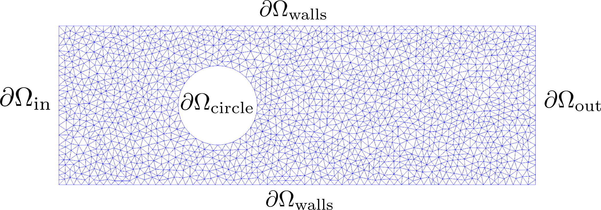
where \(\Omega\) is the domain of interest (visualised below), \(u:\Omega \to \mathbb R^2\) is the unknown velocity, \(p:\Omega \to \mathbb R\) is the unknown pressure, \(\nu\) is the viscosity, \(\alpha\) is the regularisation parameter, \(f\) denotes the value for the Dirichlet inflow boundary condition, and \(g\) is the control variable that specifies the Dirichlet boundary condition on the circle.

Physically, this setup corresponds to minimising the loss of flow energy into heat by actively controlling the in/outflow at the circle boundary. To avoid excessive control solutions, non-zero control values are penalised via the regularisation term.

Implementation

First, the dolfin and dolfin_adjoint modules are imported:

from dolfin import *
from dolfin_adjoint import *

Next, we load the mesh. The mesh was generated with mshr; see make-mesh.py in the same directory.

mesh_xdmf = XDMFFile(mpi_comm_world(), "rectangle-less-circle.xdmf")
mesh = Mesh()
mesh_xdmf.read(mesh)

Then, we define the discrete function spaces. A Taylor-Hood finite-element pair is a suitable choice for the Stokes equations. The control function is the Dirichlet boundary value on the velocity field and is hence be a function on the velocity space (note: FEniCS cannot restrict functions to boundaries, hence the control is defined over the entire domain).

V_h = VectorElement("CG", mesh.ufl_cell(), 2)
Q_h = FiniteElement("CG", mesh.ufl_cell(), 1)
W = FunctionSpace(mesh, V_h * Q_h)
V, Q = W.split()

v, q = TestFunctions(W)
x = TrialFunction(W)
u, p = split(x)
s = Function(W, name="State")
g = Function(V.collapse(), name="Control")

The Nitsche method requires the computation of boundary integrals over \(\partial \Omega_{\textrm{circle}}\). Therefore, we need to create a measure for these integrals, which will be accessible as ds(2) in the definition of the variational formulation.

class Circle(SubDomain):
    def inside(self, x, on_boundary):
        return on_boundary and (x[0]-10)**2 + (x[1]-5)**2 < 3**2

facet_marker = FacetFunction("size_t", mesh)
facet_marker.set_all(10)
Circle().mark(facet_marker, 2)

ds = ds(subdomain_data=facet_marker)

Now we define some parameters, including the Nitsche penalty parameter \(\gamma\) (typically 10), the mesh element size \(h\), the normal direction at the boundary \(n\), and the strong Dirichlet boundary conditions apart from the circle boundary where we will enforce the boundary condition via the Nitsche method.

# Set parameter values
nu = Constant(1)     # Viscosity coefficient
gamma = Constant(10)    # Nitsche penalty parameter
n = FacetNormal(mesh)
h = CellSize(mesh)

# Define boundary conditions
u_inflow = Expression(("x[1]*(10-x[1])/25", "0"))
noslip = DirichletBC(W.sub(0), (0, 0),
                     "on_boundary && (x[1] >= 9.9 || x[1] < 0.1)")
inflow = DirichletBC(W.sub(0), u_inflow, "on_boundary && x[0] <= 0.1")
bcs = [inflow, noslip]

The Dirichlet condition at the circle is enforced by the Nitsche approach. To begin with we derive the standard weak formulation of the Stokes problem: Find \(u, p\) such that for all test functions \(v, q\)

\[a(u,p; v,q) = L(u,p;v,q)\]

with

\[\begin{split}a(u,p;v,q) =&\ \nu \left<\nabla (u), \nabla (v)\right>_\Omega - \nu \left<\nabla (u) n, v\right>_{\partial \Omega_{\textrm{circle}}} \\ & - \left<p, \textrm{div} v \right>_{\Omega} + \left<p n, v\right>_{\partial \Omega_{\textrm{circle}}} - \left<q, \textrm{div} u \right>_{\Omega} \\ L(u,p;v,q) =&\ 0\end{split}\]

Note that we only need to include boundary integrals over the circle, as other boundary terms vanish due to the application of strong Dirichlet conditions.

To apply the symmetric Nitsche approach on the circle boundary, we introduce new boundary terms to the left hand side \(a\) such that the resulting problem becomes symmetric, plus the Nitsche term \(\frac{\gamma}{h} \nu \left<u,v\right>_{\partial \Omega_{\textrm{circle}}}\). Furthermore, we add the same terms to the right hand side \(L\) with \(u\) substituted by the boundary value \(g\). This yields the weak formulation:

\[\begin{split}a(u, v) =&\ \nu \left<\nabla (u), \nabla (v)\right>_\Omega - \nu \left<\nabla (u) n, v\right>_{\partial \Omega_{\textrm{circle}}} - \nu \left<\nabla (v) n, u\right>_{\partial \Omega_{\textrm{circle}}} + \frac{\gamma}{h} \nu \left<u,v\right>_{\partial \Omega_{\textrm{circle}}} \\ & - \left<p, \textrm{div} v \right>_{\Omega} + \left<p n, v\right>_{\partial \Omega_{\textrm{circle}}} - \left<q, \textrm{div} u \right>_{\Omega} + \left<q n, u\right>_{\partial \Omega_{\textrm{circle}}} \\ L(u, v) =&\ - \nu \left<\nabla (v) n, g\right>_{\partial \Omega_{\textrm{circle}}} + \frac{\gamma}{h} \nu \left<g,v\right>_{\partial \Omega_{\textrm{circle}}} + \left<q n, g\right>_{\partial \Omega_{\textrm{circle}}}\end{split}\]

In code, this becomes:

a = (nu*inner(grad(u), grad(v))*dx
     - nu*inner(grad(u)*n, v)*ds(2)
     - nu*inner(grad(v)*n, u)*ds(2)
     + gamma/h*nu*inner(u, v)*ds(2)
     - inner(p, div(v))*dx
     + inner(p*n, v)*ds(2)
     - inner(q, div(u))*dx
     + inner(q*n, u)*ds(2)
     )
L = (- nu*inner(grad(v)*n, g)*ds(2)
     + gamma/h*nu*inner(g, v)*ds(2)
     + inner(q*n, g)*ds(2)
     )

Next we assemble and solve the system once to record it with dolin-adjoint.

A, b = assemble_system(a, L, bcs)
solve(A, s.vector(), b)

Next we define the functional of interest \(J\), the optimisation parameter \(g\), and derive the create the reduced functional.

u, p = split(s)
alpha = Constant(10)

J = Functional(1./2*inner(grad(u), grad(u))*dx + alpha/2*inner(g, g)*ds(2))
m = Control(g)
Jhat = ReducedFunctional(J, m)

Now, everything is set up to run the optimisation and to plot the results. By default, minimize uses the L-BFGS-B algorithm.

g_opt = minimize(Jhat)
plot(g_opt, title="Optimised boundary")

g.assign(g_opt)
A, b = assemble_system(a, L, bcs)
solve(A, s.vector(), b)
plot(s.sub(0), title="Velocity")
plot(s.sub(1), title="Pressure")
interactive()

Results

The example code can be found in examples/stokes-bc-control in the dolfin-adjoint source tree, and executed as follows:

$ python stokes-bc-control.pystokes_bc_control.py
  ...
  At iterate    9    f=  1.98909D+01    |proj g|=  6.05347D-04

  At iterate   10    f=  1.98909D+01    |proj g|=  1.12697D-04

  At iterate   11    f=  1.98909D+01    |proj g|=  7.03065D-05

             * * *

  Tit   = total number of iterations
  Tnf   = total number of function evaluations
  Tnint = total number of segments explored during Cauchy searches
  Skip  = number of BFGS updates skipped
  Nact  = number of active bounds at final generalized Cauchy point
  Projg = norm of the final projected gradient
  F     = final function value

             * * *

     N    Tit     Tnf  Tnint  Skip  Nact     Projg        F
  14384     11     13      1     0     0   7.031D-05   1.989D+01
    F =   19.890932240156282

  CONVERGENCE: REL_REDUCTION_OF_F_<=_FACTR*EPSMCH

   Cauchy                time 0.000E+00 seconds.
   Subspace minimization time 0.000E+00 seconds.
   Line search           time 0.000E+00 seconds.

   Total User time 0.000E+00 seconds.

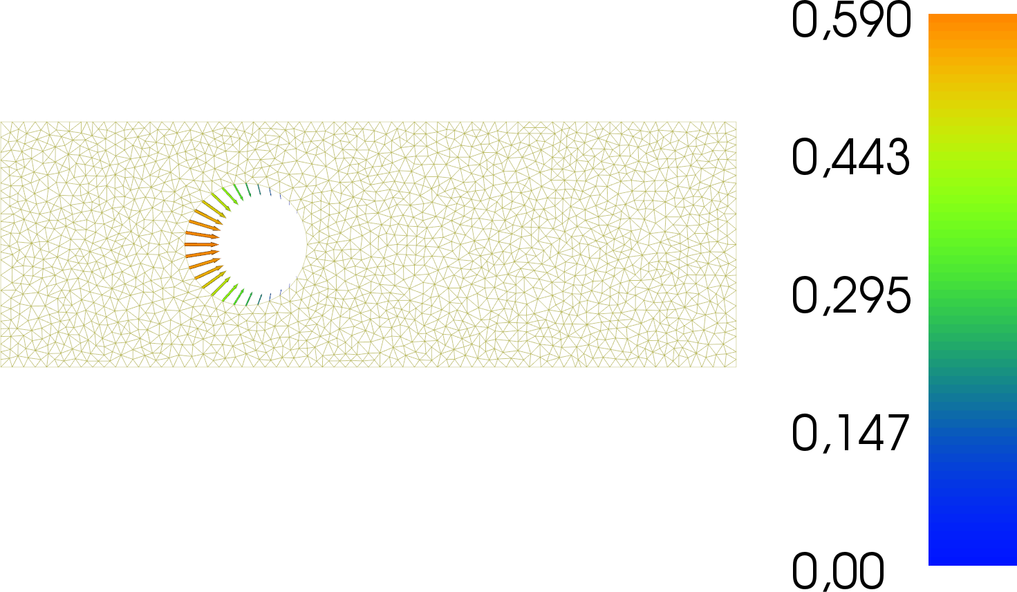
The results are visualised in the following images. The first image shows the optimised control function, i.e. the Dirichlet values on the circle boundary which minimise the loss of flow energy into heat.

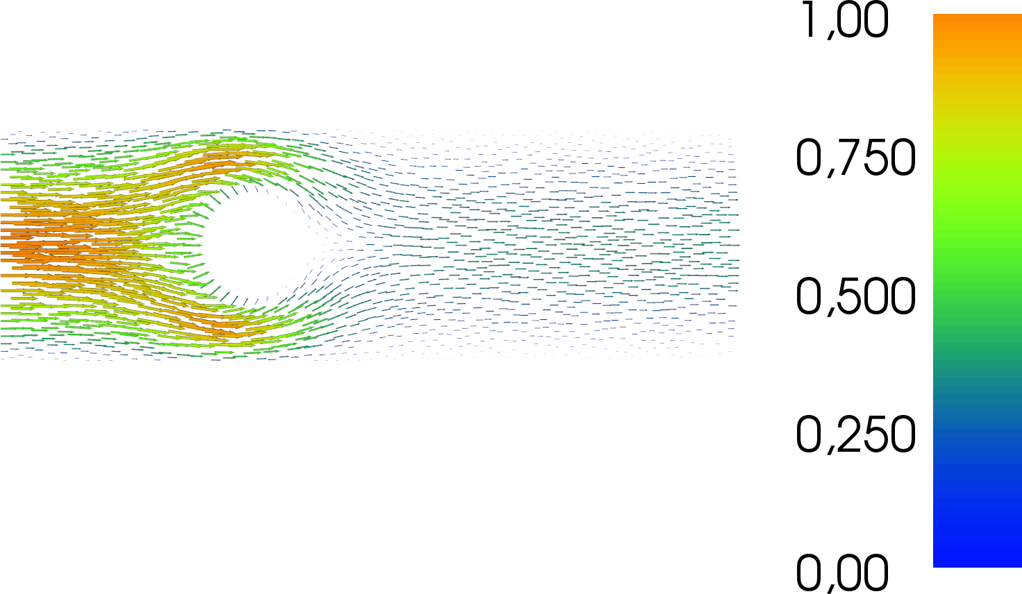
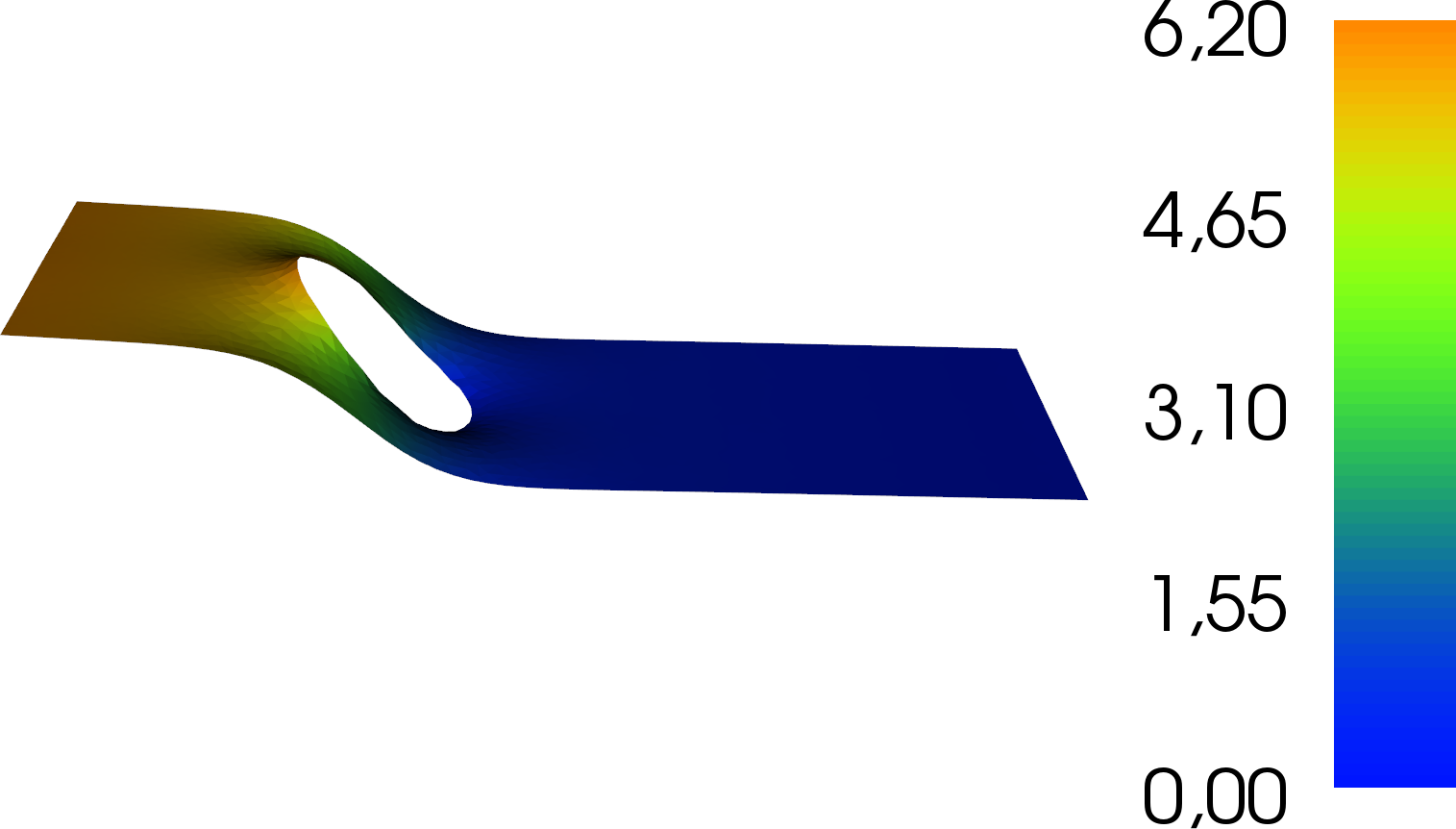
The next image shows the associated velocity:

And the final image shows the pressure:

[2E-BH07]

Y. Bazilevs and T.J.R. Hughes. Weak imposition of Dirichlet boundary conditions in fluid mechanics. Computers & Fluids, 36(1):12–26, 2007. doi:10.1016/j.compfluid.2005.07.012.

[2E-Han05]

P Hansbo. Nitsche’s method for interface problems in computational mechanics. GAMM-Mitteilungen, 28(2):183–206, 2005.

[2E-Nit71]

J. Nitsche. Über ein Variationsprinzip zur Lösung von Dirichlet-Problemen bei Verwendung von Teilräumen, die keinen Randbedingungen unterworfen sind. In Abhandlungen aus dem Mathematischen Seminar der Universität Hamburg, volume 36, 9–15. Springer, 1971. doi:10.1007/BF02995904.