
First steps
Foreword
If you have never used the FEniCS system before, you should first read their tutorial. If you’re not familiar with adjoints and their uses, see the background.
A first example
Let’s suppose you are interested in solving the nonlinear time-dependent Burgers equation:
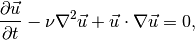
subject to some initial and boundary conditions.
A forward model that solves this problem with P2 finite elements might look as follows:
from dolfin import *

n = 30
mesh = UnitSquareMesh(n, n)
V = VectorFunctionSpace(mesh, "CG", 2)

ic = project(Expression(("sin(2*pi*x[0])", "cos(2*pi*x[1])")),  V)
u = Function(ic)
u_next = Function(V)
v = TestFunction(V)

nu = Constant(0.0001)

timestep = Constant(0.01)

F = (inner((u_next - u)/timestep, v)
   + inner(grad(u_next)*u_next, v)
   + nu*inner(grad(u_next), grad(v)))*dx

bc = DirichletBC(V, (0.0, 0.0), "on_boundary")

t = 0.0
end = 0.1
while (t <= end):
    solve(F == 0, u_next, bc)
    u.assign(u_next)
    t += float(timestep)
 You can download the source code and follow along as we
adjoin this code.
You can download the source code and follow along as we
adjoin this code.
The first change necessary to adjoin this code is to import the dolin-adjoint module after loading dolfin:
from dolfin import *
from dolfin_adjoint import *
The reason why it is necessary to do it afterwards is because
dolfin-adjoint overloads many of the dolfin API functions to
understand what the forward code is doing. In this particular case,
the solve function and
assign method have been
overloaded:
 while (t <= end):
     solve(F == 0, u_next, bc)
     u.assign(u_next)
The dolfin-adjoint versions of these functions will record each step of the model, building an annotation, so that it can symbolically manipulate the recorded equations to derive the tangent linear and adjoint models. Note that no user code had to be changed: it happens fully automatically.
In order to talk about adjoints, one needs to consider a particular functional. While dolfin-adjoint supports arbitrary functionals, let us consider a simple nonlinear example. Suppose our functional of interest is the square of the norm of the final velocity:
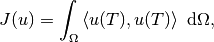
or in code:
J = Functional(inner(u, u)*dx*dt[FINISH_TIME]).
Here, multiplying by *dt[FINISH_TIME] indicates that the
functional is to be evaluated at the final time.
If the functional were to be an integral over time, one could
multiply by *dt. This requires some more annotation; see
the documentation for adj_inc_timestep. For how to express
more complex functionals, see the documentation on expressing
functionals.
The dolfin-adjoint software has several drivers, depending on
precisely what the user requires. The highest-level interface is to
compute the gradient of the functional with respect to some
Control. For example, suppose we wish to compute the
gradient of  with respect to the initial condition for
 , using the adjoint. We can do this with the following code:
dJdic = compute_gradient(J, Control(u))
where Control indicates that the
gradient should be computed with respect to the initial condition of that function. This
single function call differentiates the model, assembles each adjoint
equation in turn, and then uses the adjoint solutions to compute the
requested gradient.
Other Controls are possible. For example, to compute the
gradient of the functional with respect to the diffusivity
 :
:
dJdnu = compute_gradient(J, Control(nu))
Note that by default,
compute_gradient
deallocates all of the forward solutions it can as it goes along, to
minimise the memory footprint: however, if you try to run the adjoint
twice, it will give an error because it no longer has the necessary
forward variables:
>>> dJdic = compute_gradient(J, Control(u))
>>> dJdnu = compute_gradient(J, Control(nu))
Traceback (most recent call last):
...
libadjoint.exceptions.LibadjointErrorNeedValue: Need a value for
   w_2:1:6:Forward, but don't have one recorded.
w_2 refers to the Function u, and 1:6 means the sixth
(last) iteration associated with timestep 1; i.e., libadjoint is
telling us that it needs the terminal velocity, but it doesn’t have
it, as it’s been deallocated already in the first call to
compute_gradient. To
tell compute_gradient not
to deallocate the forward solutions as it goes along, pass
forget=False:
from dolfin import *
from dolfin_adjoint import *

n = 30
mesh = UnitSquareMesh(n, n)
V = VectorFunctionSpace(mesh, "CG", 2)

ic = project(Expression(("sin(2*pi*x[0])", "cos(2*pi*x[1])")),  V)
u = Function(ic)
u_next = Function(V)
v = TestFunction(V)

nu = Constant(0.0001)

timestep = Constant(0.01)

F = (inner((u_next - u)/timestep, v)
   + inner(grad(u_next)*u_next, v)
   + nu*inner(grad(u_next), grad(v)))*dx

bc = DirichletBC(V, (0.0, 0.0), "on_boundary")

t = 0.0
end = 0.1
while (t <= end):
    solve(F == 0, u_next, bc)
    u.assign(u_next)
    t += float(timestep)

J = Functional(inner(u, u)*dx*dt[FINISH_TIME])
dJdic = compute_gradient(J, Control(u), forget=False)
dJdnu = compute_gradient(J, Control(nu))
Observe how the changes required from the original forward code to the adjoined version are very small: with only four lines added to the original code, we are able to compute the gradient information.
If you have been following along, you can download the
adjoined Burgers’ equation code and compare your results.
Other interfaces are available to manually compute the adjoint and tangent linear solutions. For details, see the section on lower-level interfaces.
Once you have computed the gradient, how do you know if it is correct? If you were to pass an incorrect gradient to an optimisation algorithm, the convergence would be hampered or it may fail entirely. Therefore, before using any gradients, you should satisfy yourself that they are correct. dolfin-adjoint offers easy routines to rigorously verify the computed results, which is the topic of the next section.